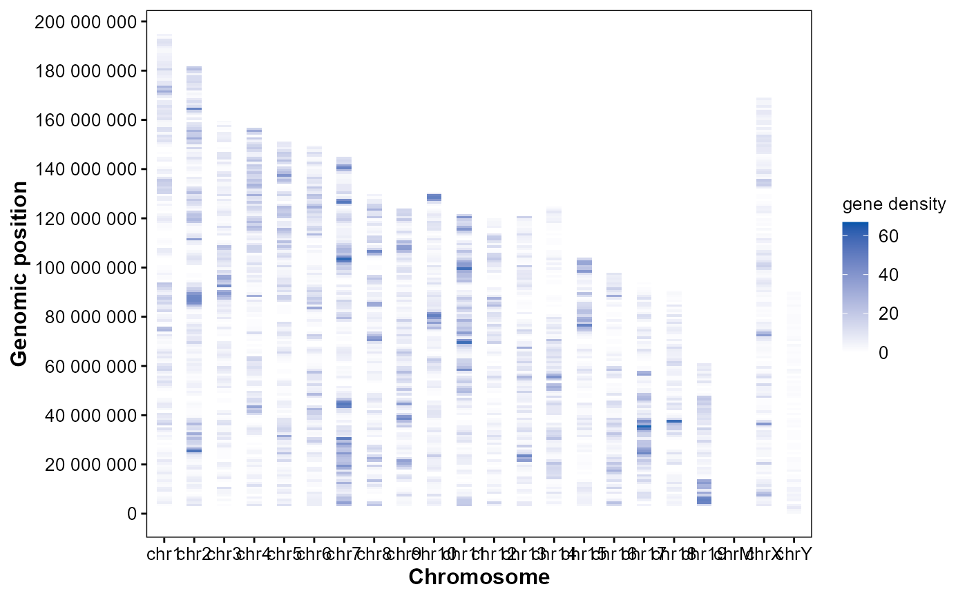
Plot genomic feature density heatmap — plot_chrom

Plot genomic feature density heatmap.

Usage

plot_chrom_heatmap(
  gff_file,
  format = "auto",
  feature = "gene",
  bin_size = 1e+06,
  orientation = "horizontal",
  palette = c("#ffffff", "#0055aa"),
  alpha = 0.9
)

Arguments

gff_file: Genomic structural annotation GFF3/GTF file path.
format: Format of GFF3/GTF file. ("auto", "gff3", "gtf").
feature: Genomic feature to quantify. ("gene", "exon", "CDS", "promoter").
bin_size: Window size (bp) for density calculation. (1e6).
orientation: Coordinate orientation. ("horizontal", "vertical").
palette: Continuous color palette for density. (c("#ffffff", "#0055aa")).
alpha: Tile alpha for density heatmap. (0.9).

Value

A ggplot object showing genomic feature density heatmap.

Author

benben-miao

Examples

# Example GFF3 file in GAnnoViz
gff_file <- system.file(
  "extdata",
  "example.gff3.gz",
  package = "GAnnoViz")

# Gene density heatmap
plot_chrom_heatmap(
  gff_file = gff_file,
  format = "auto",
  feature = "gene",
  bin_size = 1e6,
  orientation = "horizontal",
  palette = c("#ffffff", "#0055aa"),
  alpha = 0.9
)
#> Import genomic features from the file as a GRanges object ... 
#> OK
#> Prepare the 'metadata' data frame ... 
#> OK
#> Make the TxDb object ... 
#> OK
#> Coordinate system already present.
#> ℹ Adding new coordinate system, which will replace the existing one.