Plot differentially expressed genes (DEGs) hyper/hypo distributions by chromosome
Source:R/plot_deg_chrom.R
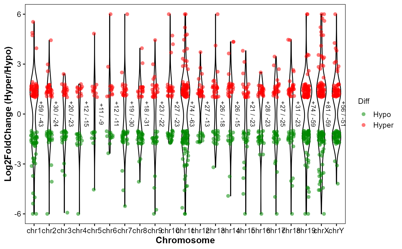
plot_deg_chrom.RdPlot differentially expressed genes (DEGs) hyper/hypo distributions by chromosomes.
Usage
plot_deg_chrom(
  deg_file,
  gff_file,
  format = "auto",
  id_col = "GeneID",
  fc_col = "log2FoldChange",
  violin_scale = "count",
  violin_border = 0.5,
  point_shape = 16,
  point_size = 2,
  jitter_width = 0.2,
  hyper_color = "#ff000088",
  hypo_color = "#00880088"
)
Arguments
- deg_file
DEG table from DESeq2 analysis.
- gff_file
Genomic structural annotation
GFF3/GTFfile path.- format
Format of GFF3/GTF file. ("auto", "gff3", "gtf").
- id_col
Gene IDs column name. ("GeneID").
- fc_col
Log2(fold change) column name. ("log2FoldChange").
- violin_scale
Violin scale mode. ("count", "area", "width").
- violin_border
Violin border width. (0.5).
- point_shape
Points shape (0-25). (16).
- point_size
Point size. (2).
- jitter_width
Horizontal jitter width. (0.2).
- hyper_color
Color for up-regulated points. ("#ff000088").
- hypo_color
Color for down-regulated points. ("#00880088").
Examples
# DEG results from DESeq2
deg_file <- system.file(
    "extdata",
    "example.deg",
    package = "GAnnoViz")

# Genomic structure annotation
gff_file <- system.file(
    "extdata",
    "example.gff3.gz",
    package = "GAnnoViz")

# Plot
plot_deg_chrom(
  deg_file = deg_file,
  gff_file = gff_file,
  format = "auto",
  id_col = "GeneID",
  fc_col = "log2FoldChange",
  violin_scale = "count",
  violin_border = 0.5,
  point_shape = 16,
  point_size = 2,
  jitter_width = 0.2,
  hyper_color = "#ff000088",
  hypo_color = "#00880088"
)
#> Import genomic features from the file as a GRanges object ...
#> OK
#> Prepare the 'metadata' data frame ...
#> OK
#> Make the TxDb object ...
#> OK