Dendrograms for multiple samples/groups clustering.
Usage
dendro_plot(
  data,
  dist_method = "euclidean",
  hc_method = "ward.D2",
  tree_type = "rectangle",
  k_num = 5,
  palette = "npg",
  color_labels_by_k = TRUE,
  horiz = FALSE,
  label_size = 1,
  line_width = 1,
  rect = TRUE,
  rect_fill = TRUE,
  xlab = "Samples",
  ylab = "Height",
  ggTheme = "theme_publication"
)
Arguments
- data
Dataframe: All genes in all samples expression dataframe of RNA-Seq (1st-col: Genes, 2nd-col~: Samples).
- dist_method
Character: distance measure method. Default: "euclidean", options: "euclidean", "maximum", "manhattan", "canberra", "binary" or "minkowski".
- hc_method
Character: hierarchical clustering method. Default: "ward.D2", options: "ward.D", "ward.D2", "single", "complete","average" (= UPGMA), "mcquitty" (= WPGMA), "median" (= WPGMC) or "centroid" (= UPGMC).
- tree_type
Character: plot tree type. Default: "rectangle", options: "rectangle", "circular", "phylogenic".
- k_num
Numeric: the number of groups for cutting the tree. Default: 3.
- palette
Character: color palette used for the group. Default: "npg", options: "npg", "aaas", "lancet", "jco", "ucscgb", "uchicago", "simpsons" and "rickandmorty".
- color_labels_by_k
Logical: labels colored by group. Default: TRUE, options: TRUE or FALSE.
- horiz
Logical: horizontal dendrogram. Default: FALSE, options: TRUE or FALSE.
- label_size
Numeric: tree label size. Default: 0.8, min: 0.
- line_width
Numeric: branches and rectangle line width. Default: 0.5, min: 0.
- rect
Logical: add a rectangle around groups. Default: TRUE, options: TRUE or FALSE.
- rect_fill
Logical: fill the rectangle. Default: TRUE, options: TRUE or FALSE.
- xlab
Character: title of the xlab. Default: "".
- ylab
Character: title of the ylab. Default: "Height".
- ggTheme
Character: ggplot2 theme. Default: "theme_publication", options: "theme_default", "theme_bw", "theme_gray", "theme_light", "theme_linedraw", "theme_dark", "theme_minimal", "theme_classic", "theme_void".
Examples
# 1. Library TOmicsVis package
library(TOmicsVis)
# 2. Use example dataset gene_expression
data(gene_expression)
head(gene_expression)
#> Genes CT_1 CT_2 CT_3 LT20_1 LT20_2 LT20_3 LT15_1 LT15_2
#> 1 transcript_0 655.78 631.08 669.89 654.21 402.56 447.09 510.08 442.22
#> 2 transcript_1 92.72 112.26 150.30 88.35 76.35 94.55 120.24 80.89
#> 3 transcript_10 21.74 31.11 22.58 15.09 13.67 13.24 12.48 7.53
#> 4 transcript_100 0.00 0.00 0.00 0.00 0.00 0.00 0.00 0.00
#> 5 transcript_1000 0.00 14.15 36.01 0.00 0.00 193.59 208.45 0.00
#> 6 transcript_10000 89.18 158.04 86.28 82.97 117.78 102.24 129.61 112.73
#> LT15_3 LT12_1 LT12_2 LT12_3 LT12_6_1 LT12_6_2 LT12_6_3
#> 1 399.82 483.30 437.89 444.06 405.43 416.63 464.75
#> 2 73.94 96.25 82.62 85.48 65.12 61.94 73.44
#> 3 13.35 11.16 11.36 6.96 7.82 4.01 10.02
#> 4 0.00 0.00 0.00 0.00 0.00 0.00 0.00
#> 5 232.40 148.58 0.00 181.61 0.02 12.18 0.00
#> 6 85.70 80.89 124.11 115.25 113.87 107.69 119.83
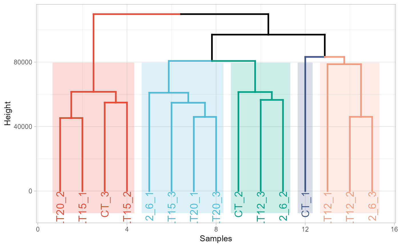
# 3. Default parameters
dendro_plot(gene_expression)
#> Registered S3 method overwritten by 'dendextend':
#> method from
#> rev.hclust vegan
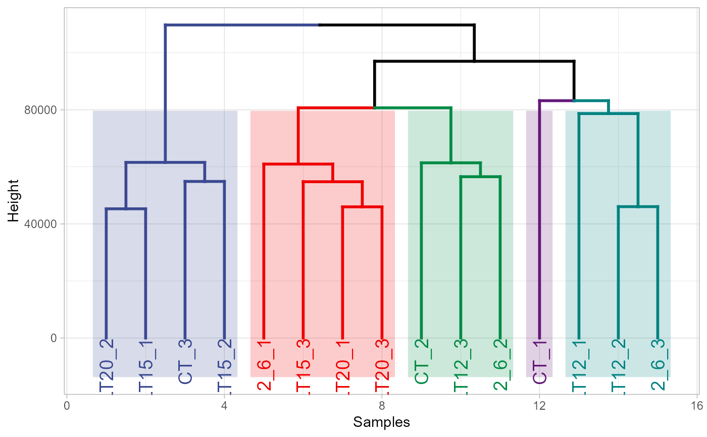
 # 4. Set palette = "aaas"
dendro_plot(gene_expression, palette = "aaas")
# 4. Set palette = "aaas"
dendro_plot(gene_expression, palette = "aaas")
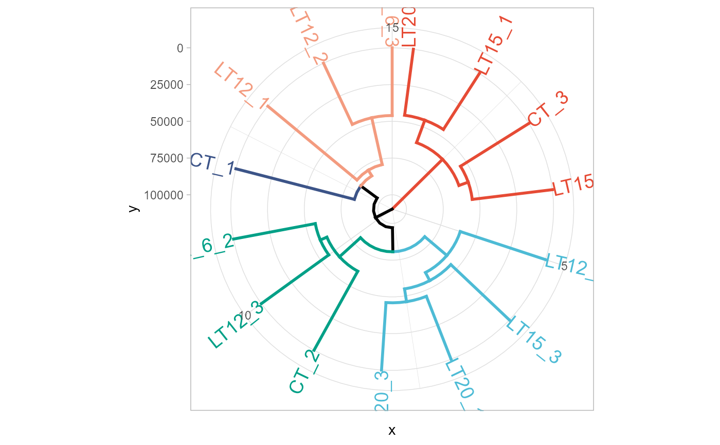
 # 5. Set tree_type = "circular"
dendro_plot(gene_expression, tree_type = "circular")
# 5. Set tree_type = "circular"
dendro_plot(gene_expression, tree_type = "circular")