Trend plot for visualizing gene expression trend profile in multiple traits.
Source:R/trend_plot.R
trend_plot.RdTrend plot for visualizing gene expression trend profile in multiple traits.
Usage
trend_plot(
  data,
  scale_method = "centerObs",
  miss_value = "exclude",
  line_alpha = 0.5,
  show_points = TRUE,
  show_boxplot = TRUE,
  num_column = 1,
  xlab = "Traits",
  ylab = "Genes Expression",
  sci_fill_color = "Sci_AAAS",
  sci_fill_alpha = 0.8,
  sci_color_alpha = 0.8,
  legend_pos = "right",
  legend_dir = "vertical",
  ggTheme = "theme_publication"
)
Arguments
- data
Dataframe: Shared degs of all paired comparisons in all groups expression dataframe of RNA-Seq. (1st-col: Genes, 2nd-col~n-1-col: Groups, n-col: Pathways).
- scale_method
Character: data scale methods. Default: "globalminmax" (global min and max values), options: "std" (standard), "robust", "uniminmax" (unique min and max values), "globalminmax", "center", "centerObs" (center observes).
- miss_value
Character: deal method for missing values. Default: "exclude", options: "exclude", "mean", "median", "min10", "random".
- line_alpha
Numeric: lines color alpha. Default: 0.50, min: 0.00, max: 1.00.
- show_points
Logical: show points at trait node. Default: TRUE, options: TRUE, FALSE.
- show_boxplot
Logical: show boxplot at trait node. Default: TRUE, options: TRUE, FALSE.
- num_column
Logical: column number. Default: 2, min: 1, max: null.
- xlab
Character: x label. Default: "Traits".
- ylab
Character: y label. Default: "Genes Expression".
- sci_fill_color
Character: ggsci color pallet. Default: "Sci_AAAS", options: "Sci_AAAS", "Sci_NPG", "Sci_Simpsons", "Sci_JAMA", "Sci_GSEA", "Sci_Lancet", "Sci_Futurama", "Sci_JCO", "Sci_NEJM", "Sci_IGV", "Sci_UCSC", "Sci_D3", "Sci_Material".
- sci_fill_alpha
Numeric: ggsci fill color alpha. Default: 0.50, min: 0.00, max: 1.00.
- sci_color_alpha
Numeric: ggsci border color alpha. Default: 1.00, min: 0.00, max: 1.00.
- legend_pos
Character: legend position. Default: "right", options: "none", "left", "right", "bottom", "top".
- legend_dir
Character: legend direction. Default: "vertical", options: "horizontal", "vertical".
- ggTheme
Character: ggplot2 themes. Default: "theme_publication", options: "theme_default", "theme_bw", "theme_gray", "theme_light", "theme_linedraw", "theme_dark", "theme_minimal", "theme_classic", "theme_void"
Examples
# 1. Library TOmicsVis package
library(TOmicsVis)
# 2. Use example dataset
data(gene_expression3)
head(gene_expression3)
#> Genes CT LT20 LT15 LT12 LT12_6
#> 1 ACAA2 39.903333 123.4366667 272.3533 359.28333 464.940000
#> 2 ACAN 14.660000 142.4800000 226.0333 316.43667 1083.523333
#> 3 ADH1 1.713333 14.8066667 12.2000 17.54333 9.343333
#> 4 AHSG 637.330000 0.0000000 0.0000 0.00000 0.000000
#> 5 ALDH2 2.490000 0.6033333 0.2700 0.13000 0.210000
#> 6 AP1S3 10.170000 27.3433333 29.1600 32.44667 44.276667
#> Pathways
#> 1 PPAR signaling pathway
#> 2 PPAR signaling pathway
#> 3 PPAR signaling pathway
#> 4 PPAR signaling pathway
#> 5 PPAR signaling pathway
#> 6 PPAR signaling pathway
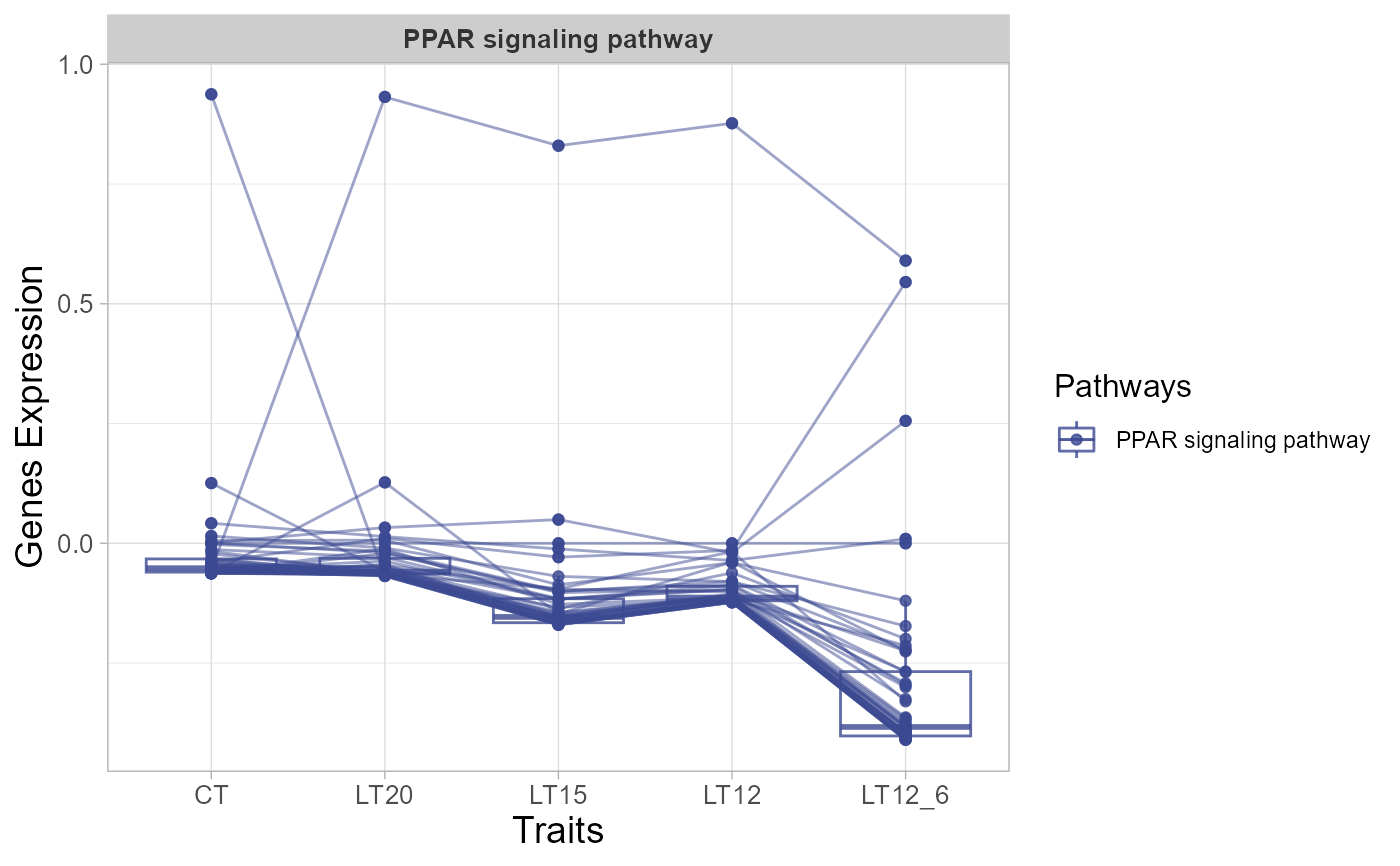
# 3. Default parameters
trend_plot(gene_expression3[1:50,])
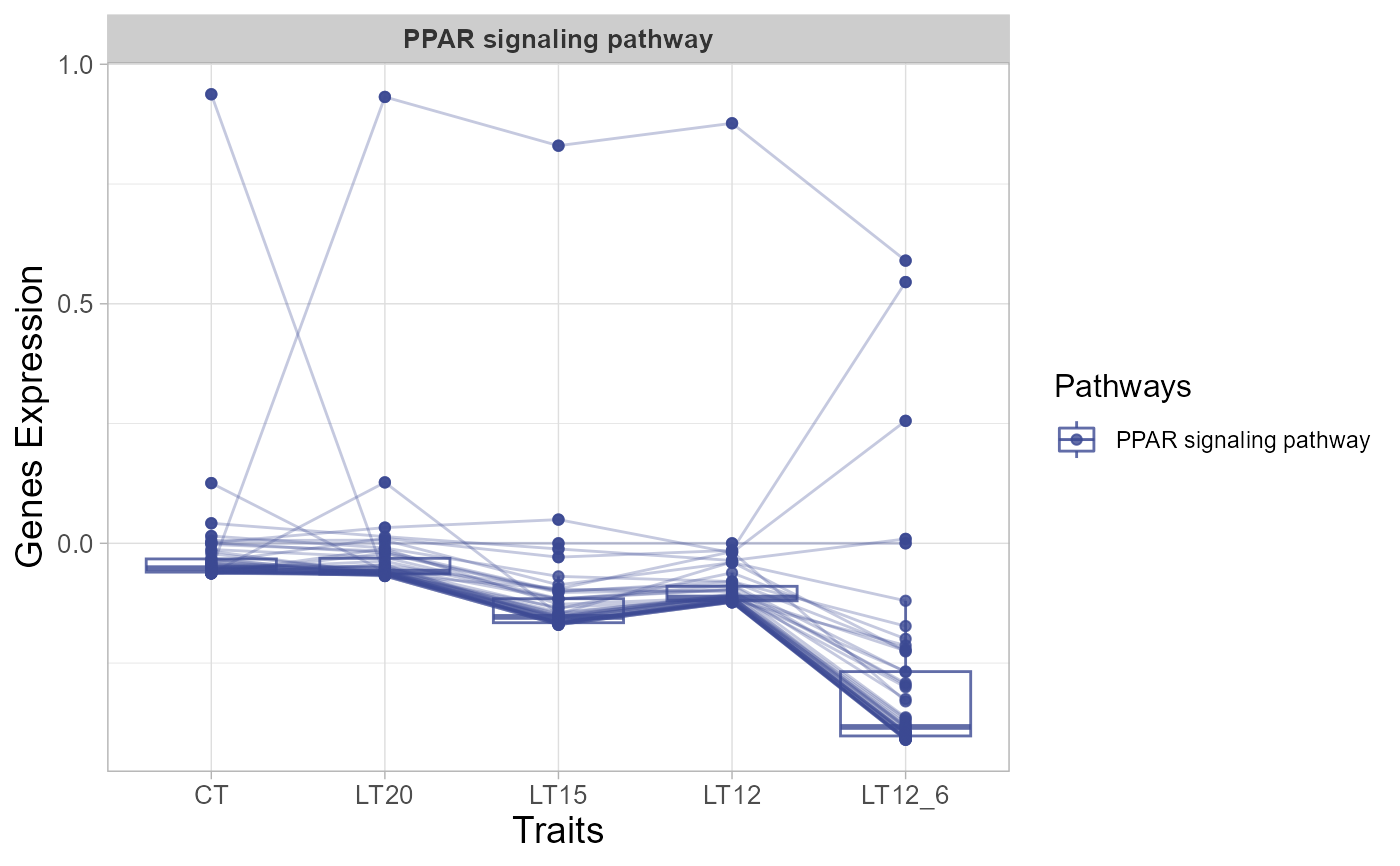
 # 4. Set line_alpha = 0.30
trend_plot(gene_expression3[1:50,], line_alpha = 0.30)
# 4. Set line_alpha = 0.30
trend_plot(gene_expression3[1:50,], line_alpha = 0.30)
 # 5. Set sci_fill_color = "Sci_NPG"
trend_plot(gene_expression3[1:50,], sci_fill_color = "Sci_NPG")
# 5. Set sci_fill_color = "Sci_NPG"
trend_plot(gene_expression3[1:50,], sci_fill_color = "Sci_NPG")
